VASP Tutorial: DFT Calculation For $\mathrm{WS_{2}}$ With SOC
Published:
The method for general PBE calculation is quite comprehensive in previous tutorials, while the DFT simulation process that requires the consideration of SOC (spin-orbital coupling) remains blank. Here in this tutorial, we’re going to summerize the process for the DFT calculation of WS2 considering SOC effect.
DFT without SOC
The process of DFT calculation (PBE) using VASP has been quite clear in the following reference: https://tamaswells.github.io/VASPKIT_manual/manual0.73/vaspkit-manual-0.73.html#header-n46
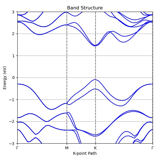
We use monolayer $\mathrm{WS_{2}}$ in this tutorial. The DFT result without SOC is shown below:
DFT with SOC
There are two steps, for calculating DFT with SOC effect. Firstly, we calculate the SCF (static self-consistent functional) DFT. The INCAR script should be like this:
Global Parameters
ISTART =  1            (Read existing wavefunction, if there)
ISPIN  =  2            (Non-Spin polarised DFT)
#ICHARG =  11         (Non-self-consistent: GGA/LDA band structures)
LREAL  = .FALSE.       (Projection operators: automatic)
# ENCUT  =  400        (Cut-off energy for plane wave basis set, in eV)
# PREC   =  Accurate   (Precision level: Normal or Accurate, set Accurate when perform structure lattice relaxation calculation)
LWAVE  = .FALSE.        (Write WAVECAR or not)
LCHARG = .TRUE.        (Write CHGCAR or not)
ADDGRID= .TRUE.        (Increase grid, helps GGA convergence)
# LVTOT  = .TRUE.      (Write total electrostatic potential into LOCPOT or not)
# LVHAR  = .TRUE.      (Write ionic + Hartree electrostatic potential into LOCPOT or not)
# NELECT =             (No. of electrons: charged cells, be careful)
# LPLANE = .TRUE.      (Real space distribution, supercells)
# NWRITE = 2           (Medium-level output)
# KPAR   = 2           (Divides k-grid into separate groups)
# NGXF    = 300        (FFT grid mesh density for nice charge/potential plots)
# NGYF    = 300        (FFT grid mesh density for nice charge/potential plots)
# NGZF    = 300        (FFT grid mesh density for nice charge/potential plots)

Static Calculation
ISMEAR =  0            (gaussian smearing method)
SIGMA  =  0.05         (please check the width of the smearing)
LORBIT =  11           (PAW radii for projected DOS)
NEDOS  =  2001         (DOSCAR points)
NELM   =  60           (Max electronic SCF steps)
EDIFF  =  1E-08        (SCF energy convergence, in eV)
#LSORBIT = .TRUE.
The INCAR file could be generated in vaspkit and then modified specifically for ISPIN = 2 and LWAVE = .FALSE. (Ban the generation of WAVECAR).
Run the following command in the terminal:
mpirun -genv FI_PROVIDER=mlx vasp_std
The second step for SOC. The INCAR is as follows:
Global Parameters
ISTART =  1            (Read existing wavefunction, if there)
ISPIN  =  2            (Non-Spin polarised DFT)
ICHARG =  11        (Non-self-consistent: GGA/LDA band structures)
LREAL  = .FALSE.       (Projection operators: automatic)
# ENCUT  =  400        (Cut-off energy for plane wave basis set, in eV)
# PREC   =  Accurate   (Precision level: Normal or Accurate, set Accurate when perform structure lattice relaxation calculation)
LWAVE  = .FALSE.        (Write WAVECAR or not)
LCHARG = .TRUE.        (Write CHGCAR or not)
ADDGRID= .TRUE.        (Increase grid, helps GGA convergence)
# LVTOT  = .TRUE.      (Write total electrostatic potential into LOCPOT or not)
# LVHAR  = .TRUE.      (Write ionic + Hartree electrostatic potential into LOCPOT or not)
# NELECT =             (No. of electrons: charged cells, be careful)
# LPLANE = .TRUE.      (Real space distribution, supercells)
# NWRITE = 2           (Medium-level output)
# KPAR   = 2           (Divides k-grid into separate groups)
# NGXF    = 300        (FFT grid mesh density for nice charge/potential plots)
# NGYF    = 300        (FFT grid mesh density for nice charge/potential plots)
# NGZF    = 300        (FFT grid mesh density for nice charge/potential plots)

LSORBIT = .TRUE.
Here we copy the CHARCAR file from the previous step and set ICHARG = 11 to read the charge infomation from the last step. Then we set LSORBIT = .TRUE. to enable the SOC calculation.
We can generate KPATH.in in vaspkit, and replace the content of KPATH.in file to the KPOINTS file.
Run the following command in the terminal:
mpirun -genv FI_PROVIDER=mlx vasp_nclHere, a python script written by myself is provided for the automatic process of DFT calculation of a set of MD trajectories.
from ase.io import read, write
from ase.io.lammpsdata import write_lammps_data
from math import sin,cos
import numpy as np
from ase.io import read, write
import os
import shutil
import pexpect
import subprocess
class snapshot():
"""this is to create a snapshot related object
Args:
Variable (_type_): _description_
"""
def __init__(self, shot_index):
self.shot_index = shot_index
self.file_prefix = 'dump'
self.file_suffix = 'lammpstrj'
self.source_POTCAR_dir = '/home/sliang/2x2_WS2/VASP'
self.source_INCAR_SCF_dir = '/home/sliang/2x2_WS2/VASP/INCAR_SCF'
self.source_INCAR_SO_dir = '/home/sliang/2x2_WS2/VASP/INCAR_SO'
def snap_create_folder(self):
print("Creating Snapshot Folder.")
path = f"./{self.shot_index}"
os.makedirs(path, exist_ok=True)
path = f"./{self.shot_index}/step2"
os.makedirs(path, exist_ok=True)
def convert_trac2vasp(self):
print("Converting POSCAR file format.")
# This function is to convert file format to vasp format and store it in a new folder.
file = f'./{self.file_prefix}.{self.shot_index}.{self.file_suffix}'
atoms = read(file, index=0)
write(f'{self.shot_index}/POSCAR', atoms)
write(f'{self.shot_index}/step2/POSCAR', atoms)
def DFT_calculation(self):
# In this method we only apply PBE calculation, because the HSE method is freaking time-consuming.
# Firstly we generate related IN files for vasp
parent_file_dir = os.getcwd() # get the dir of parent file.
snapshot_folder_dir = os.path.join(parent_file_dir,str(self.shot_index)) # the directory of the snapshot folder
os.chdir(snapshot_folder_dir)
run_vasp_command = ["mpirun", "-genv", "FI_PROVIDER=mlx", "vasp_std"]
run_vasp_ncl_command = ["mpirun", "-genv", "FI_PROVIDER=mlx", "vasp_ncl"]
################ DFT Phase I: SCF Calculation ###################
# Copy the INCAR file
print("Generating INCAR File.")
source_INCAR_SCF = os.path.join(self.source_INCAR_SCF_dir,'INCAR')
shutil.copy(source_INCAR_SCF, snapshot_folder_dir)
# Copy the POTCAR file
print("Generating POTCAR File.")
source_POT_W = os.path.join(self.source_POTCAR_dir,'POTCAR_W')
source_POT_S = os.path.join(self.source_POTCAR_dir,'POTCAR_S')
source_POT = os.path.join(self.source_POTCAR_dir,'POTCAR')
shutil.copy(source_POT_W, snapshot_folder_dir)
shutil.copy(source_POT_S, snapshot_folder_dir)
shutil.copy(source_POT, snapshot_folder_dir)
# Generate the KPOINTS file
print("Generating KPOINTS File.")
vasp_kit_auto = pexpect.spawn('vaspkit')
vasp_kit_auto.expect(r'------------>>')
vasp_kit_auto.sendline('1')
vasp_kit_auto.expect(r'------------>>')
vasp_kit_auto.sendline('102') # Generate KPOINTS File for SCF Calculation
vasp_kit_auto.expect(r'------------>>')
vasp_kit_auto.sendline('2') # Gamma Scheme
vasp_kit_auto.expect('Input Kmesh-Resolved Value \(in Units of 2\*PI/Angstrom\):')
vasp_kit_auto.sendline('0.04')
vasp_kit_auto.expect('-->> \(02\) Written KPOINTS File!')
output_after_kpoints_selection = vasp_kit_auto.before.decode('utf-8')
print("OUPUT:")
print(output_after_kpoints_selection)
vasp_kit_auto.close()
# Conduct Phase I PBE calculation
subprocess.run(run_vasp_command)
################ DFT Phase II: SOC Calculation ###################
snapshot_folder_dir_step2 = os.path.join(snapshot_folder_dir,str(step2)) # the directory of the step2 folder
os.chdir(snapshot_folder_dir_step2)
# Copy the INCAR file
print("Generating INCAR File.")
source_INCAR_SO = os.path.join(self.source_INCAR_SO_dir,'INCAR')
shutil.copy(source_INCAR_SO, snapshot_folder_dir_step2)
# Copy the POTCAR file
print("Generating POTCAR File.")
shutil.copy(source_POT_W, snapshot_folder_dir_step2)
shutil.copy(source_POT_S, snapshot_folder_dir_step2)
shutil.copy(source_POT, snapshot_folder_dir_step2)
vasp_kit_auto = pexpect.spawn('vaspkit')
vasp_kit_auto.expect(r'------------>>')
vasp_kit_auto.sendline('3') # Band-Path Generator
vasp_kit_auto.expect(r'------------>>')
vasp_kit_auto.sendline('302') # 2D structure
vasp_kit_auto.expect('-->> \(03\) Written KPATH.in File for Band-Structure Calculation.')
output_after_kpoints_selection = vasp_kit_auto.before.decode('utf-8')
print("OUPUT:")
print(output_after_kpoints_selection)
vasp_kit_auto.close()
subprocess.run('cp -f KPATH.in KPOINTS', shell=True) # Using KPATH.in as new KPOINTS
# Copy the CHGCAR file
source_CHG = os.path.join(snapshot_folder_dir,'CHGCAR')
shutil.copy(source_CHG, snapshot_folder_dir_step2)
# Conduct Phase II PBE calculation
subprocess.run(run_vasp_ncl_command)
vasp_kit_auto = pexpect.spawn('vaspkit')
vasp_kit_auto.expect(r'------------>>')
vasp_kit_auto.sendline('21') # Read the band structure from the eigen energy file
vasp_kit_auto.expect(r'------------>>')
vasp_kit_auto.sendline('211') # Generate band structure.
vasp_kit_auto.expect('-->> \(10\) Written BAND_GAP File!')
output_after_kpoints_selection = vasp_kit_auto.before.decode('utf-8')
print("OUPUT:")
print(output_after_kpoints_selection)
vasp_kit_auto.close()
os.chdir(parent_file_dir)
def main():
for i in range(1,1001):
# 126-250 snapshots, before this was 100 steps.
index = (100+i)*500
print(f"Processing {index} snapshot.")
snapshot_i = snapshot(index)
# create folder
snapshot_i.snap_create_folder()
# convert POSCAR file format
snapshot_i.convert_trac2vasp()
# DFT Calculation
snapshot_i.DFT_calculation()
if __name__ == "__main__":
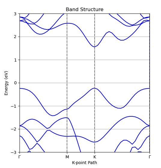
main()The band structure for monolayer WS2 considering SOC effect is demonstrated as below: